Introduction to information channels
Information processing is part of our everyday life. From reading your alarm clock in the morning to your dinner decision this evening, you’re in a constant bath of information. Despite the ability to process this information via your senses, interpreting this information physically and mathematically can seem overwhelming. Nevertheless, understanding the laws of nature requires a rigorous and exhaustive approach to modeling these processes. Those who study information sciences, have developed a series of mathematical tools to help understand the inter-workings behind how information transfers from inputs to outputs. These transfers, are aptly named information channels.
Scientists are not the only ones who use information channels. In fact, as alluded above, they are a part of your every day life. An obvious information channel may be entering your pin number into an ATM. In this process, transfer of information that was stored in your brain into the ATM, enabled the machine to grant access for managing your banking. To Quantum Information Scientists, the processes that take place on the smallest of scales, like the photons exiting the ATM screen and entering your eyes, have complicated yet fascinating information channels that processes classical and quantum information.
Just as with other fields of physics, classical and quantum information channels follow separate rules. The quantum revolution of the 1920s brought with it a confusing perspective of how we are to view the governing mechanics of the micro-world. Up until that moment, nature could be described by a set of deterministic rules. Only limited by the complexity of each system and the ignorance of the observer. The quantum founding fathers showed that at the smallest of scales, nature is fundamentally determined by probabilities.
The probabilistic nature of quantum mechanics would thus play a lofty role in how we understand information. Imagine entering your pin number into a quantum mechanical ATM, only to get rejected fifty percent of the time. Rejected not due to some noise or interference, but instead some inherent property that governs the interactions taking place inside the ATM. We can see that these two ATMs process different types of information and subsequently need to construct different types of information channels. However, certain properties of these information channels will be analogous to each other. Therefore, in this article, we dive first into a more familiar domain of classical information channels while preparing to understand the more complicated but coinciding quantum information channels.
The aim of this article, is to introduce some of the tools necessary to understand the properties of information channels. While the mathematics is deep and complex, I do my best to keep it self-contained as much as possible, with the intent to offer a broader audience the ideas behind information theory. Regardless, readers can skip the math as it appears, without loss of generality. For those inclined to dig deeper into information channels, you will find these helpful [1,2].
Classical Information Channels
As mentioned previously, complexity of a classical system can shroud its deterministic properties. Probabilities are often deployed as a simplification to these complex systems. While there is nothing quantum about flipping a fair coin, the fact that quantum theory is probabilistic, allows us to draw similar allusions by following such a system. To unpack the information hidden in this random process of coin flipping, we need a theory to measure information as it changes through these classical processes. For that, we turn to Shannon’s[3] information theory.
Shannon’s theory is best understood with the usage of bits. A bit is a single piece of information that describes the state of an object. Consider the above example of a fair coin. The state of the coin can be described by assigning the value of zero to heads and one to tails. Therefore, reading out the bit is equivalent to measuring the state of the coin. To measure the information of a system[4], we first consider the Shannon entropy \(H(X)\) given by,
\begin{equation} \label{shannon entropy} H(X) = \sum_x -p_X(x)\log p_X(x) \end{equation}
with probability distribution \(p_X(x)\). \(H(x)\) will measure the randomness or surprise in the output of the system. If we consider our above example of the fair coin we expect a Shannon Entropy of one, which is the maximum amount of uncertainty for this system. This can easily be seen by replacing the fair coin with a weighted coin. A weighted coin with two-thirds probability of heads and one-third probability of tails, has a Shannon Entropy of 0.918. A weighted coin with nine-tenths probability of heads and one-tenth tails will yields 0.469. As the coin gets more weighted, the uncertainty in the result of the coin flip goes down, and subsequently the measure of Shannon Entropy does as well. Generally, we can say if \(x\) is the probability of obtaining heads, the probability of obtaining tails is \(1-x\) and eq. \eqref{shannon entropy} becomes, \begin{equation} H(X) = x\log x + (1-x)\log(1-x). \end{equation}
We can see in figure 1, that the information content of \(X\) is maximized when both the events are equally likely. This makes sense because having equal probability outcomes, makes the task of guessing the hardest. So in essence, the entropy is closely related to the contents of the information channel.
For readers who enjoy the mathematics (others can skip this paragraph), Shannon entropy specifically measures information content of the random variable \(X\). If we refer to this “surprise” or “randomness” of an outcome \(x\) as the information content \(i(x)\), and define it as \(i(x) = \log(\frac{1}{p(x)}) = -\log(p(x))\). This measurement has the property that it is high for low probability outcomes and low for high probability outcomes. Moreover, this also has another desirable property of “additivity” i.e. the information content of two outcomes \(x\) and \(y\) get added since the joint probability \(p(x,y) = p(x).p(y) \implies i(x,y) = -\log(p(x)p(y)) = -\log(p(x)) - \log(p(y)) = i(x) + i(y)\). Thus, the total information content of the random variable \(X\) can be written as the weighted average of the information of possible outcomes.
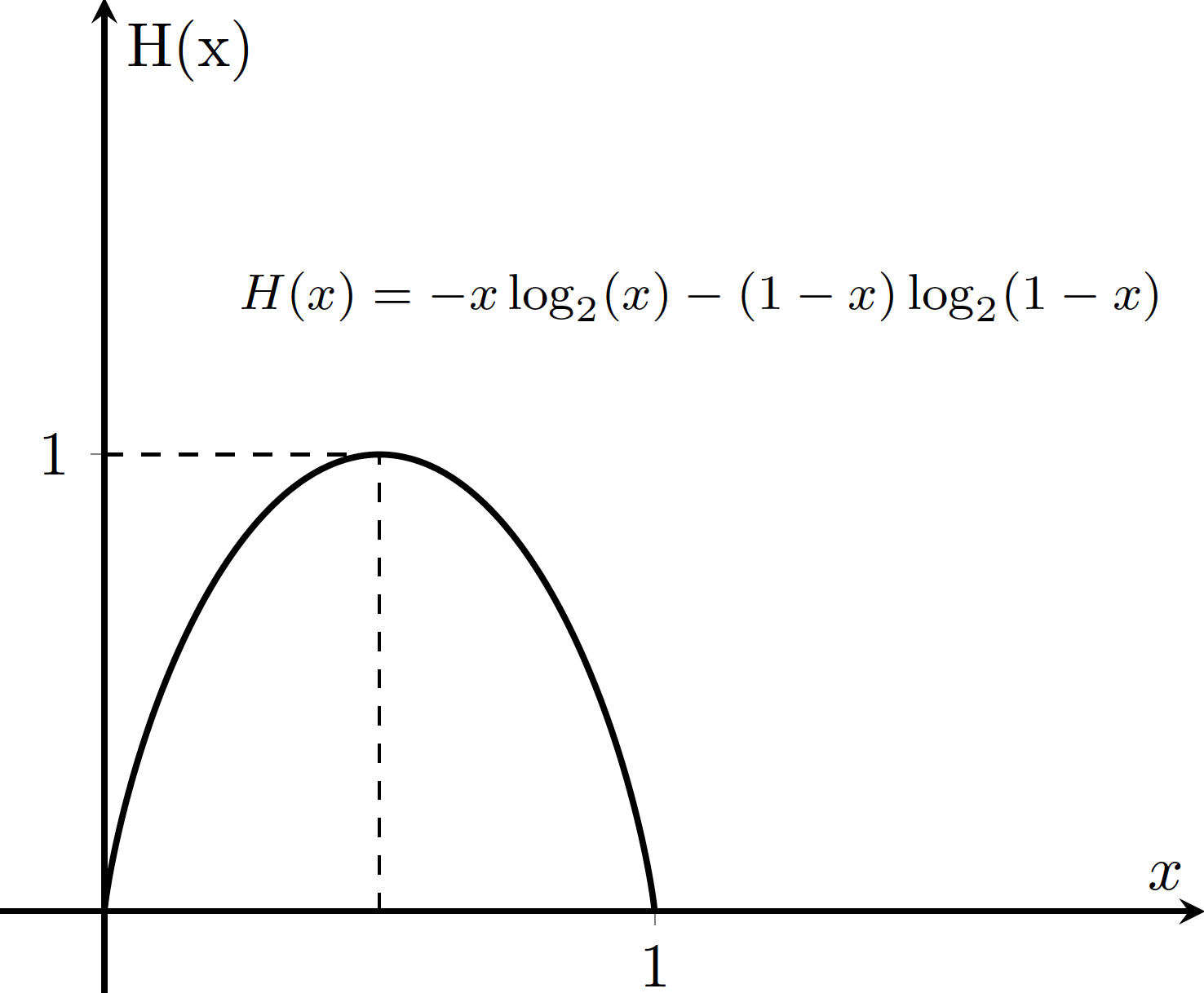
Fig 1: Graphical representation of H(x) for our fair-coin flipping system. Notice the maximum entropy occurs when our probability \(x = 1/2\)
For both the classical and the quantum case of information channels, we will model a very simple operation that has purpose both in classical and quantum computing. For the classical system we will use a flip operation. The flip operation will take our input bit and flip the value of it. For instance, our fair coin modeled with heads as zero and tails as one, will do just as it says. Flip the side of the coin from its initial configuration to the opposite. Figure 2 gives a pictorial representation of this process.
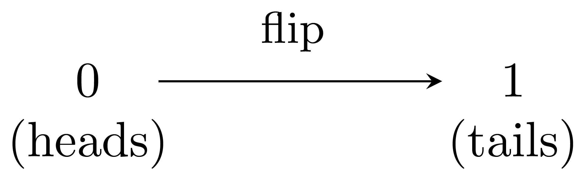
Fig 2: A simple classical information channel that shows a flip operation acting on a coin. The coin is initially in state of heads but the flip operation changes this to tails.
A useful calculation in information theory is Channel Capacity, which is a measure of information loss (or conversely propagated) through our circuit. Information lost is often do to the noisiness of a channel. Noise is attributed to unwanted interactions and will affect the input states by altering them. For instance, a sender Alice and a receiver Bob may be attempting to communicate classically. Choosing a noisy channel to save resources could alter the inputs enough that Bob would be unable to decipher the original message Alice has sent. If instead of a fair coin, suppose Alice has access to a set of random variables \(X\). She encodes a message onto the elements of \(X\) and sends it via some noisy channel to Bob who receives a set of random variables \(Y\) to decipher. Our aim now must be to mathematically evaluate the channel that led from \(X\) to \(Y\). This will show if the channel reliably transferred Alice’s message. Pictorially this is shown in figure 3.
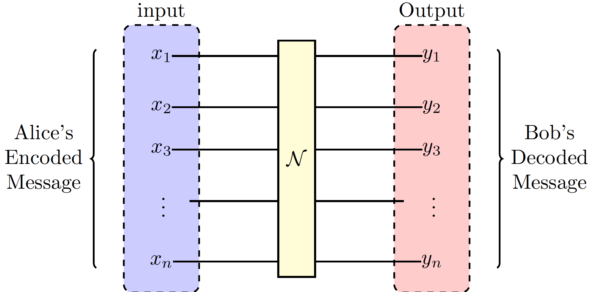
Fig 3: Alice’s message is encoded into the elements \(x_i\) where it is passed through some noisy channel \(\mathcal{N}\) and later deciphered by Bob.
After the information transfer, Bob has access to \(Y\), and the amount of his randomness/surprise about \(X\) is quantified by the Conditional Entropy. Mathematically this has the shape, \begin{equation} \label{Conditional Entropy} H(Y|X) = -\sum{x,y}p{Y|X}(y|x)\log \left( \frac{p*{Y|X}(y|x)}{p_Y(y)} \right) \end{equation} where \(p*{X,Y}(x,y)\) is an expression of the multiplicity of probability namely, \(p_{X,Y}(x,y)=p_X(x)p_Y(y)\). Notice that \(H(X) \geq H(X|Y)\), and subsequently \(I(X;Y) \geq 0\). Here these probabilities are a result of the interactions within the noisy quantum channels. The measure of how much information Bob recovers, can be expressed as the Mutual Information \(I(X;Y)\), where \begin{equation}\label{Mutual Information} I(X;Y) = H(Y)-H(Y|X). \end{equation} The mutual information in essence quantifies the similarity or correlations between the random variables of Alice and Bob. This is because \(H(Y|X)\) quantifies the amount of error due to noise. In a perfect channel this value is zero because \(Y\) is fully aware of how \(X\) will change.
Up until this point, we have very purposefully not discussed the contents of the noisy information channels. We want to have a means to describe an information channel either classically or quantum mechanically, but the contents of the channels may be messy and hard to understand. This is where Channel Capacity comes into play. Channel Capacity uses information to quantifiably measure the reliability of an information channel \(\mathcal{N}\). The means as to which the information passes through that channel is equivalent to knowledge of the information given and received. After all, the channel is a probabilistic mapping of the set \(X\) onto the set \(Y\), \begin{equation} \mathcal{N}:p_{Y|X}(y|x). \end{equation} Under this construction, we define the Channel Capacity as,
\begin{equation} \mathcal{C}(\mathcal{N}) = \max{p{X}(x)}I(X;Y) \end{equation}
which has a physical interpretation such that, if Alice can arrange her information in a way that allows a maximal amount of correlation with Bobs, then this is the upper bound to the capacity of the channel. Using what we learned about information, we can quantify the capacity of a channel which will help identify if these channels are efficient uses of resources.
Quantum Information Channels
A quantum channel is a linear, completely positive, and trace preserving mapping corresponding to a physical evolution. This is a fancy way of saying that it too, is a probabilistic mapping from initial states to final states. Yet something deeper is going on here. The probabilities involved the information transfer is not necessarily due to our inability to evaluate a complex system. Instead, the mechanics are fundamentally probabilistic. This leads to a relationship deeper than correlation, Entanglement.
Entanglement is the signature of a quantum information channel. We illustrate entanglement through a comparison to classical correlation. Suppose Alice and Bob are presented with two colored balls red and blue. The ball’s identities are concealed and Alice randomly selects one of the balls. Without looking, she departs for a far away star system. Upon arrival, Alice glances at her ball and notices the color is red. She can infer through correlation that Bob’s ball is blue. Now, suppose we repeat the experiment but, instead of balls we use perpetually spinning quantum coins. Ignoring how this is possible, let’s say that these quantum coins are arranged such that, if Alice measures heads, Bob’s coin will also measure heads. Similarly, if Alice measures tails, Bob’s will too! Alice ventures to the same far off system, quantum coin in hand, and measures her coin to which she instantly knows the measurement of Bob’s coin. The difference here is subtle. Our first experiment, involved a measurement early on, only random due to the ignorance of the observer, Alice. Throughout the voyage, Alice’s ball remained red, regardless of her knowledge. So to an outside observer, there was no surprise when she gets to her destination. A measurement of red was inevitable. The hidden information in the correlated state lived as classical information, only hidden by Alice’s inability to measure the color. Whereas, for experiment two, the states remained truly and fundamentally random up until the very moment Alice takes the measurement.
The key to this entanglement, is the connection between the two quantum coins which we have conveniently hidden in the phrase ``Ignoring how this is possible”. Coincidentally, it is very possible in the realm of quantum mechanics. While, there is no classical analogy to explain why the coin-flip outcomes are correlated in this specific way, we don’t have to look far to find an example of this in nature. The spins of a pair of electrons can be entangled in such a fashion. If we prepare our electrons to be in an entangled state, measuring the spin of one electron can directly inform us of the spin of another. An instance of this in quantum computing is known as a “Bell Pair” and will come in handy in the proceding paragraphs.
Entanglement, while mysterious in many ways, is a fundamental ingredient in quantum mechanics and is necessary for successful quantum computing. Similar to our classical bit, we introduce a quantum bit or qubit, that plays the same role as arbiter of information, but for quantum systems. If we assign the spin of the electron to a value of our qubit we can create a similar arrangement for information propagation. I should remind the reader that the math moving forward can seem a bit terse. Nevertheless, one should be able to skip the math and still gain an intuitive understanding of these concepts.
For our purposes, lets assign spin up to our qubit \(\ket{0}\), and spin-down to \(\ket{1}\)\footnote{For those who are unfamiliar with this language. You need only associate the assignments behind the qubits for this article. While the math is rich and rewarding, it can be exhaustive and we will not be exploring that here.} We can then construct the state of our entangled pair (a Bell State), \begin{equation} \label{entangled state} \ket{\psi} = \frac{\ket{0}\ket{0} + \ket{1}\ket{1}}{\sqrt{2}} \end{equation} where the coefficient of \(\frac{1}{\sqrt{2}}\) guarantees that \(50\%\) of the time we will measure both spin-up and \(50\%\) of the time we will measure both spin down.
Now that our descriptive states are set up as qubits, we can begin to evaluate the information in our states. Lets, first establish a parallel to our Shannon Entropy. It may surprise you that quantum mechanical entropy came first, this was accomplished by John von Neumann in 1932. Nevertheless, our von Neumann entropy has a similar form to the Shannon Entropy,
\begin{equation} \label{von Neumann entropy} S(\rho) = -Tr(\rho\log \rho) \end{equation}
where \(\rho\) is a density matrix whose purpose is to describe, in entirety, the probabilities and states of our system. If these states are eigenstates (eigenstates are states we can measure eg. spin-up and spin-down) then our density matrix takes the appearance of \(\rho = \sum_j n_j \ket{j}\bra{j}\) with \(\ket{j}\) denoting an eigenstate, and we can simplify equation \eqref{von Neumann entropy} to,
\begin{equation} \label{von Neumann entropy eigenstates} S(\rho) = -\sum_j n_j \log n_j \end{equation}
where \(n_j\) is the probability of measuring an eigenstate. But what does this quantify? In essence, this quantifies the purity of the state. While purity has some analogous meaning to classical information, we should press on with our development of quantum information and maybe a more intuitive understanding will present itself. By now you have probably noticed that equations \eqref{shannon entropy} and \eqref{von Neumann entropy eigenstates} are mostly identical. That changes quickly when we introduce Quantum Mutual Information.
To understand Quantum Mutual Information, lets give Alice one qubit and Bob another. We can entangle them such that our input state matches that of equation \eqref{entangled state}. We can then model the mutual information between Alice’s and Bob’s qubits as,
\begin{equation} I(A:B) = S(\rhoA) + S(\rho_B) - S(\rho{AB}) \end{equation}
where \(\rho_A = Tr_B (\rho)\) and \(\rho_{AB}\) is the density matrix describing the state of the Alice’s qubit. Tracing over part of the system, in essence ignores that part of the system. When we trace over Bob’s information we are focused solely on the information of Alice. The physical interpretation of mutual information is thus a quantifiable measurement of the entanglement shared between Alice and Bob. For a highly entangled state such as our bell state, we find a value of two which indicates a maximum entanglement between the two qubits. While quantum mutual information is insightful for understanding entanglement between states, these states remain as initial states. We have made a modification to our system between the classical and quantum cases. The modification is the usage of Bob. In our classical noisy channel arrangement, Bob received some data \(Y\) from Alice whose input was \(X\). The classical mutual information was a correlation between input and output. Therefore, We need another tool that is analogous to classical mutual information, that will evaluate how a quantum channel could alter this entanglement. Luckily, we’ll find a familiar analogy to classical mutual information.
The flow of quantum information is quantifiable by how much entanglement passes from the initial state to the final state. Quantum Coherent information is a quantitative measurement of this transfer. To understand it better, lets bring in a third qubit belonging to Carla. Let’s suppose Alice and Carla entangle their qubits together and create a Bell Pair like that of eq. \eqref{entangled state}. Bob’s qubit is initially in a \(\ket{0}\) (spin-up) state with \(100\%\) probability. We now define a quantum channel from Alice to Bob where we aim to pass the entanglement. A popular quantum channel that is well known to preserve entanglement is done using a SWAP gate. The SWAP gate will do just as it says; swap the values of Alice’s and Bob’s qubits and with it the information associated. Figure 4 shows this quantum information channel, outlining the SWAP of entanglement from Alice’s qubit to Bob’s.
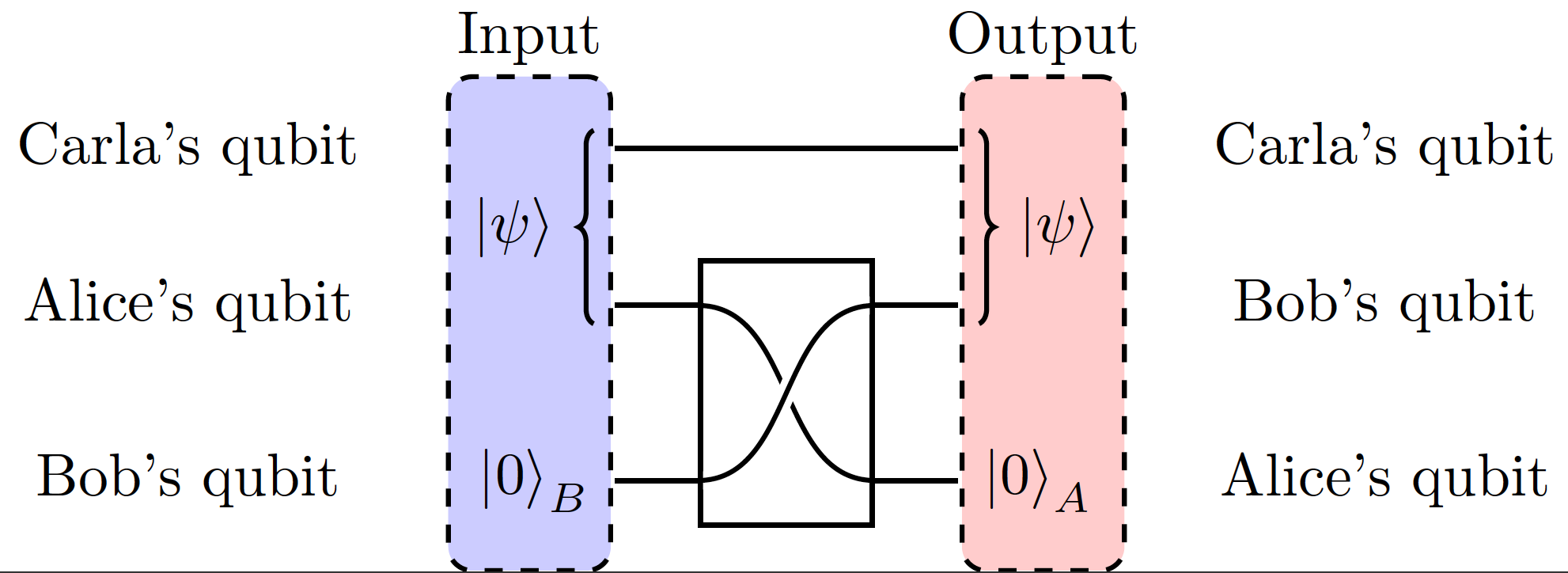
Fig 4: Alice and Carla initially have an entangled bell pair. After the SWAP gate is carried out Carla and Bob are now entangled and Alice is in the \(\ket{0}\) state.
We can now define our quantum coherent information as,
\begin{equation} IC(\rho{in,AB},\Xi) = S(\rho{out,B})-S(\rho{out,BC}). \end{equation} where, \(\rho_{in,AB}\) is the input to the channel and \(\Xi\) is the channel itself. One should note here, that the Channel \(\Xi\) is equivalent to \(\rho_{out,B}\). The difference in notations is that \(\Xi\) expresses the operators that make up the channel, and their acting on the initial states. Whereas, \(\rho_{out,B}\) is the output state which is a result of this channel. This is because \(\Xi\), mathematically is a mapping from initial states to final states. The analogy to the classical mutual information (Eq. \eqref{Mutual Information}) should be more evident now, and as we did in the classical case, we elevate this to the Quantum Channel Capacity by taking,
\begin{equation} Q(\Xi) = \max{\rho{in,AB}}IC(\rho{in,AB},\Xi). \end{equation}
Just as it was in classical information theory, the channel capacity is a measurement of reliability in transferring quantum information (ie. entanglement). So long as entanglement continues to be the best metric of a quantum computer, measuring the propagation of this entanglement, remains to be an important calculation as we further progress quantum computers.
We have spoken in detail about two channels of information, yet there remains two more. Channels that change Classical information to Quantum information (This is a process that creates entanglement) and vice versa (Measurement). These channels are handled differently, and subsequently will have to wait until future writing.
[1] M. M. Wilde, “Preface to the second edition,” Quantum Information Theory, p. xi–xii
[2] L. Gyongyosi, S. Imre, and H. V. Nguyen, “A survey on quantum chan- nel capacities,” IEEE Communications Surveys & Tutorials, vol. 20, no. 2, p. 1149-1205, 2018.
[3] Named after Claude Shannon, a mathematician and engineer who is often referred to as the “father of information theory”.
[4] We will be using \(\log_2\) for the entirety of this post for consistency.
Enjoy Reading This Article?
Here are some more articles you might like to read next: